
Context & Why
Semantic vector search is not a silver bullet for production Retrieval-Augmented Generation (RAG). Dense embeddings easily capture high-level conceptual intent, colloquial phrasing, and cross-lingual meaning. But they fall apart on precise technical inputs. Feed an embedding model an exact SKU like SKU-4821-X, a Jira ticket ID like SEC-4091, or a PostgreSQL error like 42P01. It will often hallucinate relevance or return vaguely related documentation instead of the exact match.
Standard keyword retrieval solves this precision problem. PostgreSQL’s native Full-Text Search (FTS) leverages inverted indexes to nail verbatim terms in milliseconds. The catch? It is completely blind to synonyms and user phrasing. Search for "how to repair a flat tyre", and an FTS index indexed on documents mentioning "fixing a punctured tire" yields zero hits.
Hybrid search bridges this divide. You run both lexical and vector queries concurrently, then combine the top hits into a unified candidate list.
Blending their raw scores, however, is a notorious engineering trap. Vector distances (cosine distance ranging from 0.0 to 2.0) follow a totally different statistical distribution than lexical scores like ts_rank (unbounded floating-point numbers). Setting heuristic weights like 0.7 * vector + 0.3 * fts breaks the moment you add new documents or swap embedding models.
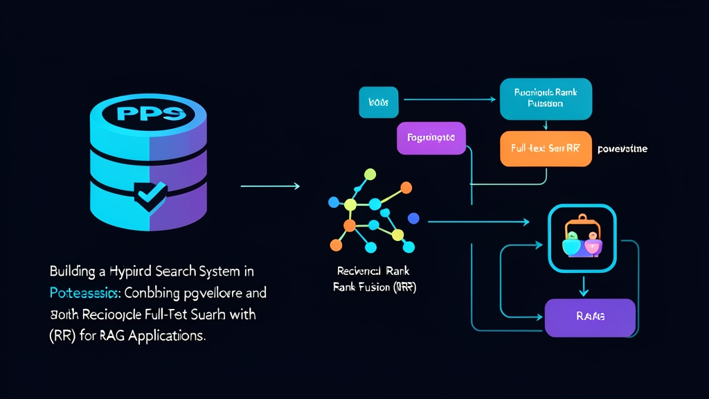
Reciprocal Rank Fusion (RRF) bypasses manual score calibration. Instead of balancing arbitrary relevance scores, RRF evaluates where each document ranks across each retrieval mechanism. The formula is refreshingly simple:
RRF_Score(d) = Σ (1 / (k + rank(d)))Here, rank(d) is the item’s 1-based position in a result list, while k is a smoothing constant. Information retrieval benchmarks typically set k = 60 to prevent outlier #1 rankings from dominating. Consider a document that finishes #1 in vector search and #4 in full-text search.
Its composite score is (1 / (60 + 1)) + (1 / (60 + 4)) = 0.01639 + 0.01562 = 0.03201. Documents ranking high across both engines rise quickly to the top. Meanwhile, documents discovered by only one pipeline still get a fair shot at the final prompt context.
Consolidating vectors and text inside PostgreSQL also saves your infrastructure. You eliminate dual-write race conditions, avoid synchronizing third-party vector databases like Pinecone or Qdrant, and keep transaction boundaries intact.
Installation
You need PostgreSQL 15 or 16 alongside the pgvector extension. Docker offers the cleanest path for local development and CI testing:
# Start PostgreSQL 16 with pgvector pre-installed
docker run -d \
  --name postgres-hybrid \
  -e POSTGRES_USER=appuser \
  -e POSTGRES_PASSWORD=secretpassword \
  -e POSTGRES_DB=rag_knowledgebase \
  -p 5432:5432 \
  pgvector/pgvector:pg16
For bare-metal Ubuntu 22.04 or 24.04 servers, grab the pre-compiled binaries directly from the official PGDG repository:
sudo apt update
sudo apt install -y postgresql-16-pgvector
Connect to your target database via psql and register the extension:
CREATE EXTENSION IF NOT EXISTS vector;Configuration
A production hybrid schema pairs raw text with two search engines: a generated tsvector column for keyword lookups and a fixed-dimension vector column for embeddings.
1. Schema Definition
CREATE TABLE documents (
    id BIGSERIAL PRIMARY KEY,
    title TEXT NOT NULL,
    content TEXT NOT NULL,
    tsv TSVECTOR GENERATED ALWAYS AS (
        setweight(to_tsvector('english', coalesce(title, '')), 'A') ||
        setweight(to_tsvector('english', coalesce(content, '')), 'B')
    ) STORED,
    embedding VECTOR(1536) -- Matches OpenAI text-embedding-3-small
);
The GENERATED ALWAYS AS ... STORED clause computes lexical tokens automatically on every INSERT or UPDATE. Using setweight assigns priority ‘A’ to title matches over body matches (‘B’), giving headline hits a natural ranking advantage.
2. Indexing Strategies
Low latency matters. Without dedicated indexes, PostgreSQL scans 500,000 rows sequentially for both queries, tanking API response times:
-- Generalized Inverted Index (GIN) for lexical filtering
CREATE INDEX idx_documents_tsv ON documents USING GIN(tsv);

-- Hierarchical Navigable Small World (HNSW) index for cosine distance
CREATE INDEX idx_documents_embedding_hnsw ON documents
USING hnsw (embedding vector_cosine_ops)
WITH (m = 16, ef_construction = 64);
Stick with HNSW over IVFFlat for production RAG collections. IVFFlat requires batch pre-training and drops recall when documents are added dynamically. HNSW builds iteratively, delivering over 95% recall out of the box with predictable latency.
3. Ingesting Data
Cleaning raw exports takes time. If you need to quickly convert CSV dumps to structured JSON for bulk inserts, browser-based utilities like toolcraft.app/en/tools/data/csv-to-json parse files locally without sending sensitive payloads over the network. Once structured, insert documents using PostgreSQL’s COPY command or parameterized batch inserts in Python.
4. The Reciprocal Rank Fusion (RRF) Query
You can execute RRF entirely inside PostgreSQL using Common Table Expressions (CTEs) and ROW_NUMBER(). This query pulls the top 60 candidates from both sides and fuses them into a calibrated top-10 result set:
WITH vector_candidates AS (
    SELECT
        id,
        title,
        content,
        ROW_NUMBER() OVER (ORDER BY embedding <=> '[0.012, -0.045, ... fill 1536 floats ... ]'::vector) AS rank
    FROM documents
    ORDER BY embedding <=> '[0.012, -0.045, ... fill 1536 floats ... ]'::vector
    LIMIT 60
),
text_candidates AS (
    SELECT
        id,
        title,
        content,
        ROW_NUMBER() OVER (ORDER BY ts_rank_cd(tsv, plainto_tsquery('english', 'database connection timeout')) DESC) AS rank
    FROM documents
    WHERE tsv @@ plainto_tsquery('english', 'database connection timeout')
    ORDER BY ts_rank_cd(tsv, plainto_tsquery('english', 'database connection timeout')) DESC
    LIMIT 60
)
SELECT
    COALESCE(v.id, t.id) AS id,
    COALESCE(v.title, t.title) AS title,
    COALESCE(v.content, t.content) AS content,
    (
        COALESCE(1.0 / (60 + v.rank), 0.0) +
        COALESCE(1.0 / (60 + t.rank), 0.0)
    ) AS rrf_score
FROM vector_candidates v
FULL OUTER JOIN text_candidates t ON v.id = t.id
ORDER BY rrf_score DESC
LIMIT 10;
Notice the FULL OUTER JOIN. It preserves documents retrieved by only one method while giving overlapping matches the benefit of additive scores.
5. Python Retrieval Function for RAG
Here is an end-to-end integration using modern psycopg (v3). Notice we format the embedding list into a PostgreSQL vector literal string:
import psycopg
from psycopg.rows import dict_row

def hybrid_search(
    db_url: str,
    query_text: str,
    query_embedding: list[float],
    limit: int = 5
) -> list[dict]:
    # Convert float array to pgvector literal '[0.012,-0.045,...]'
    vector_str = f"[{','.join(map(str, query_embedding))]}"

    sql = """
    WITH vector_candidates AS (
        SELECT id, title, content,
               ROW_NUMBER() OVER (ORDER BY embedding <=> %s::vector) AS rank
        FROM documents
        ORDER BY embedding <=> %s::vector
        LIMIT 60
    ),
    text_candidates AS (
        SELECT id, title, content,
               ROW_NUMBER() OVER (ORDER BY ts_rank_cd(tsv, plainto_tsquery('english', %s)) DESC) AS rank
        FROM documents
        WHERE tsv @@ plainto_tsquery('english', %s)
        ORDER BY ts_rank_cd(tsv, plainto_tsquery('english', %s)) DESC
        LIMIT 60
    )
    SELECT
        COALESCE(v.id, t.id) AS id,
        COALESCE(v.title, t.title) AS title,
        COALESCE(v.content, t.content) AS content,
        (
            COALESCE(1.0 / (60 + v.rank), 0.0) +
            COALESCE(1.0 / (60 + t.rank), 0.0)
        ) AS rrf_score
    FROM vector_candidates v
    FULL OUTER JOIN text_candidates t ON v.id = t.id
    ORDER BY rrf_score DESC
    LIMIT %s;
    """

    with psycopg.connect(db_url, row_factory=dict_row) as conn:
        with conn.cursor() as cur:
            cur.execute(
                sql,
                (vector_str, vector_str, query_text, query_text, query_text, limit)
            )
            return cur.fetchall()
Verification & Monitoring
After standing up your pipeline, validate retrieval relevance and profile query latency under concurrent traffic.
Validating Retrieval Behavior
Run these two sanity checks against your index to confirm RRF ranks both modalities sensibly:
- The Exact SKU/Code Test: Query for a distinctive identifier like
ORA-00942orERR-CONN-503. The text pipeline should place the exact log entry at rank #1, outmuscling any semantic drift from the embedding model. - The Conceptual Synonym Test: Search using an abstract prompt without direct keyword matches, such as "how do I prevent connection exhaustion in high concurrency web services?". Confirm that guides explaining connection poolers like PgBouncer rank at the top via the vector route.
Analyzing Query Plans
Inspect the execution path inside psql using EXPLAIN (ANALYZE, BUFFERS):
EXPLAIN (ANALYZE, BUFFERS)
WITH vector_candidates AS (...) ...
Look for three key checkpoints in the output:
- The text candidate CTE should show
Bitmap Index Scan on idx_documents_tsv. If you seeSeq Scan, review yourwork_memand verify thatenable_seqscanis not forced. - The vector candidate CTE should report
Index Scan using idx_documents_embedding_hnsw. - Overall execution time should stay between 4ms and 15ms on an indexed table of 500,000 documents.
Monitoring and Cache Tuning
HNSW graphs crave memory. If your server is forced to fetch index segments from slow NVMe or block storage on every query, latencies will jump from 8ms to well over 120ms.
-- Check disk footprint of your documents table and indexes
SELECT
    c.relname AS object_name,
    pg_size_pretty(pg_relation_size(c.oid)) AS table_size,
    pg_size_pretty(pg_total_relation_size(c.oid)) AS total_size
FROM pg_class c
JOIN pg_namespace n ON n.oid = c.relnamespace
WHERE n.nspname = 'public' AND c.relname = 'documents';
For an index with 250,000 1536-dimensional vectors, an HNSW index consumes approximately 1.8 GB of RAM. Tune your postgresql.conf to make sure it fits into cache comfortably:
# Ensure shared_buffers covers active tables and HNSW index structures
shared_buffers = 4GB

# Provide working memory for window functions and CTE sorts
work_mem = 64MB

# Set HNSW search depth (default is 40; 80-100 gives >98% recall at ~10ms latency)
# You can also set this dynamically per connection: SET hnsw.ef_search = 100;
hnsw.ef_search = 80
Keeping both your relational state and vector embeddings in PostgreSQL strips unnecessary complexity from your RAG stack. You get ACID safety, zero data drift, and sub-15ms hybrid retrieval without operating a single external vector microservice.